Quick start

Loading dependencies

using Agate
using Agate.Library.Light
using OceanBioME
using OceanBioME: Biogeochemistry
using Oceananigans
using Oceananigans.Fields: FunctionField
using Oceananigans.Units
using CairoMakie

Model setup

First, we construct our ecosystem model. Here, we use a default 2 phytoplankton, 2 zooplankton Agate.jl-NiPiZD ecosystem model.

bgc = Agate.Models.NiPiZD.construct()
using Agate.Introspection: tracer_names

# Inspect the required tracer names.
println(tracer_names(bgc))

[:N, :D, :P_1, :P_2, :Z_1, :Z_2]

The bundled NiPiZD family is assembled from the same component/process compiler used by direct ModelDefinition construction. Model with mixotrophy introduces defining a model directly from components, named processes, and a keyed parameter block.

Next, we define a light field using Oceananigans and wrap it with OceanBioME's prescribed-PAR interface. Here we use Agate's seasonal PAR helper at 10 m depth:

grid = BoxModelGrid()
clock = Clock(; time=zero(grid))
PAR = FunctionField{Center,Center,Center}(CyclicalPAR(-10), grid; clock)
light_attenuation = PrescribedPhotosyntheticallyActiveRadiation(PAR)

These two models are then combined using OceanBioME.jl

bgc_model = Biogeochemistry(bgc; light_attenuation=light_attenuation)

full_model = BoxModel(; grid, clock, biogeochemistry=bgc_model)

And finally simulated using Oceananigans.jl

set!(full_model; N=7.0, P_1=0.01, Z_1=0.01, P_2=0.1, Z_2=0.01, D=0.01)

simulation = Simulation(full_model; Δt=240minutes, stop_time=1095days)

filename = "quick_start.jld2"

simulation.output_writers[:fields] = JLD2Writer(
    full_model,
    full_model.fields;
    filename=filename,
    schedule=TimeInterval(1day),
    overwrite_existing=true,
)

run!(simulation)

[ Info: Initializing simulation...
┌ Warning: error ArgumentError("a group or dataset named grid is already present within this group") thrown when trying to serialize the grid at serialized/grid
└ @ Oceananigans.OutputWriters ~/.julia/packages/Oceananigans/9oDU5/src/OutputWriters/jld2_writer.jl:251
[ Info:     ... simulation initialization complete (1.809 seconds)
[ Info: Executing initial time step...
[ Info:     ... initial time step complete (186.228 μs).
[ Info: Simulation is stopping after running for 5.868 seconds.
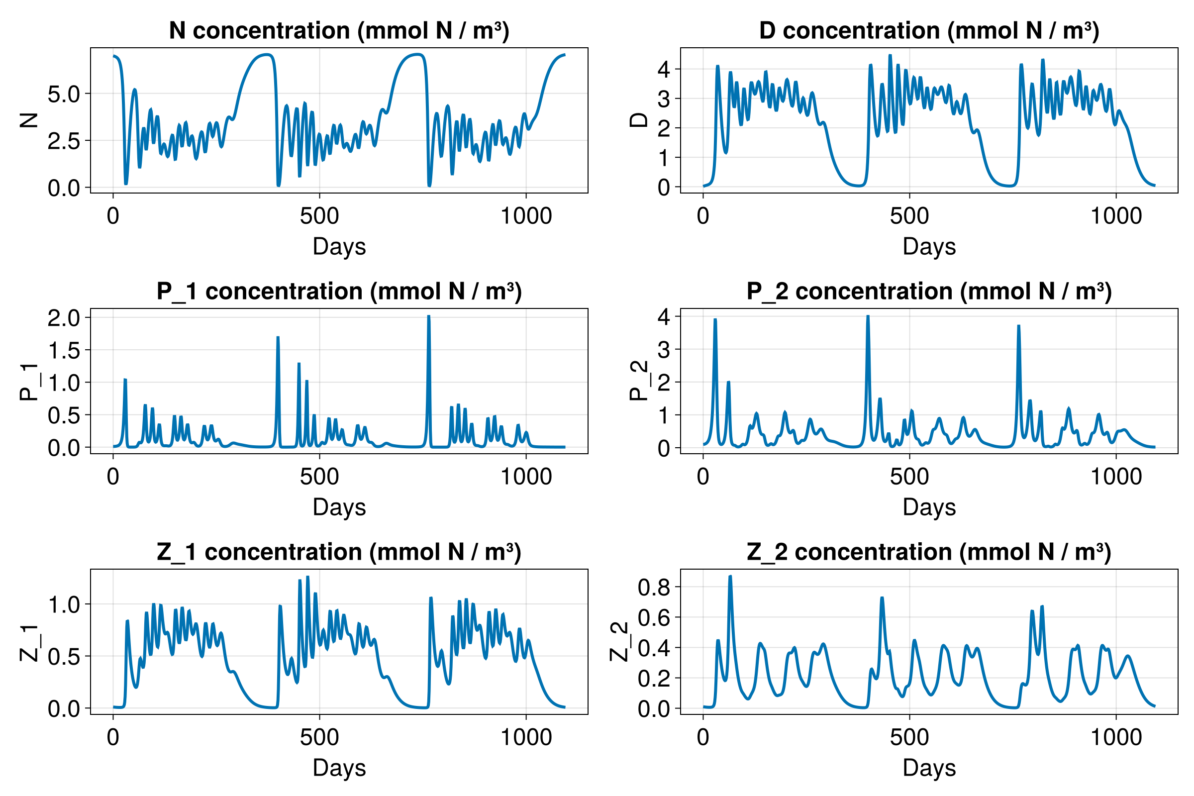
[ Info: Simulation time 1095 days equals or exceeds stop time 1095 days.

Plotting

tracer_syms = tracer_names(bgc)

# Extract data for plotting
timeseries = (;
    (s => FieldTimeSeries(filename, string(s))[1, 1, 1, :] for s in tracer_syms)...
)

# Create a figure
times = FieldTimeSeries(filename, string(first(tracer_syms))).times

fig = Figure(; size=(1200, 800), fontsize=24)

axs = []
for (idx, sym) in enumerate(tracer_syms)
    ax = Axis(
        fig[floor(Int, (idx - 1) / 2), Int((idx - 1) % 2)];
        ylabel=string(sym),
        xlabel="Days",
        title="$(sym) concentration (mmol N / m³)",
    )
    push!(axs, ax)
    lines!(ax, times / day, getproperty(timeseries, sym); linewidth=3)
end

fig